

LiteLinear 0.3.0: Accelerating Video Generation DiT with Low-Rank Linear Compression

Practical inference acceleration for production video diffusion models on NVIDIA and AMD.
TL;DR
LiteLinear is a drop-in inference acceleration library that compresses linear layers in video generation Diffusion Transformers (DiTs) using calibration-aware low-rank decomposition combined with quantization. It targets all large linear operations in the transformer, both feed-forward networks (FFN) and attention projections (Q, K, V, O), without retraining the model.
- Proof-of-concept on LTX-2 FFN: 22.5% faster transformer compute, 11.5% peak memory reduction, 7.6% faster end-to-end inference.
- Version 0.3.0 on LTX-2.3 22B: up to 8.6% end-to-end speedup on NVIDIA, ~7% on AMD MI300X warm eager, and 10%+ with LiteAttention.
- The release adds offline CLI conversion, LoRA-aware decomposition, AMD FP8 support, and persistent autotune caching.
LiteLinear repository: https://github.com/moonmath-ai/LiteLinear
LiteLinear can increase the throughput of the projection layers by up to 1.6×, depending on the choice of rank. Choosing a lower rank causes slightly lower VRAM usage and minimal video degradation, if the rank is chosen carefully and adapted to the particular model. For LTX-2, we found that applying a slightly higher rank to the to_k projection in the first denoising stage preserves video quality best.
LiteLinear 0.3.0 Update
Since the initial release of LiteLinear, we have continued to refine its integration with real-world video generation pipelines. Version 0.3.0 maintains the core approach — offline low-rank decomposition combined with an FP8 residual — while improving usability, testability, and deployment across LTX-2, NVIDIA, and AMD platforms.
The conversion workflow is now centered on a dedicated offline CLI/API process. A source checkpoint can be provided directly to the converter, which produces a LiteLinear checkpoint as a distinct artifact. Production runs then load pre-converted checkpoints in the same way they load other model artifacts.
This release also improves support for LTX-2, especially the two-stage distilled LoRA pipeline. When LoRA weights are part of inference, LiteLinear can incorporate the LoRA update before decomposition:
W_fused = W_dense + scale * LoRA
LiteLinear(W_fused) = A @ B + FP8(Q)
That lets the decomposed FFN layers represent the effective weights used in dense pipelines while preserving LiteLinear's inference performance.
A major part of 0.3.0 is AMD optimization. ROCm support now uses AMD's native FP8 format, e4m3fnuz, and the runtime path has been tuned closer to CUDA performance. Casting and conversion overhead dropped from roughly 25–30% of runtime to under 10% on reprofiled LTX-2.3 workloads.
- NVIDIA: up to 8.6% end-to-end speedup compared to dense.
- AMD: up to approximately 7% end-to-end speedup in warm eager execution.
- LiteAttention integration increases that to 10%+.
Persistent autotuning cache support on both platforms can eliminate cold-start overhead, especially in short second-stage runs. In one measured stage-2 run on MI300X, the initial step dropped from 8.42s to 3.09s, and total execution time decreased from 155.3s to 149.7s.
The Approach: Calibration-Aware Low-Rank Decomposition + Quantization
The projection layers make up a substantial part of the compute time spent on a forward pass of the transformer. After attention is optimized, they must be handled next in order to achieve a substantial speedup.
LiteLinear compresses each large linear layer by combining two ideas:
- Low-rank decomposition: approximate a large weight matrix
Was the product of two much smaller matricesAandB - Quantization: store the approximation error (remainder) in low precision (FP8 today; FP4 on the roadmap)
The key insight, borrowed from SVDQuant, is that a naive low-rank approximation misses which directions of W actually matter at runtime. LiteLinear corrects for this by collecting input statistics from real calibration data first, then decomposing in a space that reflects how the model is actually used.[1]
Why This Works on Any Linear Layer
The algorithm depends only on the shape of the weight matrix and a sample of inputs seen during normal operation. It has no dependence on the surrounding architecture, the specific model family, or the training procedure.
Any nn.Linear(in, out) layer in any DiT can be a target. LiteLinear ships with built-in support for FFN layers and attention Q/K/V/O projections, and exposes a simple API so you can target custom layer types in your own model.
How It Works (Step by Step)
Step 1: Collect Calibration Data
We run the model on a sample of real prompts and collect per-layer input statistics to characterize typical activation structure.
For each linear layer, we compute:
R = E[x * x^T]
For 2048-dimensional inputs, each autocorrelation matrix has 4 million entries. Across many
layers, memory grows quickly, so we compute R incrementally:
# Pseudocode for incremental autocorrelation
R_sum = zeros((dim, dim))
N = 0

for batch in calibration_data:
    x = get_activations(batch)  # Shape: [batch, seq_len, dim]
    x_flat = x.reshape(-1, dim) # Flatten to [N_samples, dim]
    R_sum += x_flat.T @ x_flat  # Accumulate outer product
    N += x_flat.shape[0]

R = R_sum / N
Step 2: Compute Effective Weights
We use calibration statistics to transform the original weight matrix into a form that is easier to compress:
W_effective = W @ R^(1/2)This reweights columns by practical usage, improving how efficiently SVD can approximate the matrix for real workloads.
Step 3: Decompose
W_effective = U @ S @ V^TWe keep the top-r singular components:
W_low_rank_eff = U[:, :r] @ S[:r] @ V[:r, :]^TStep 4: Handle the Remainder
Remainder = W - W_low_rankThis residual is quantized to 4-bit or 8-bit formats.
Step 5: Inference
def forward(x):
    # Low-rank path (full precision, small matrices)
    y_lowrank = A @ (B @ x)

    # Remainder path (quantized)
    y_remainder = Q_quantized @ x

    return y_lowrank + y_remainder + bias
Quantization Options
Current production format on Hopper:
FP8 E4M3
- Bits: 8 (4 exponent, 3 mantissa)
- Range: approximately +/-448
- Pros: native H100 tensor core support, strong accuracy
- Cons: 2x memory versus FP4
Planned formats for LiteLinear on Blackwell and future Hopper support include NVFP4 E2M1 and MXFP4.
The Fun Part: Multiply-Free FP4
For non-native FP4 support, NVFP4's limited value set allows replacing floating-point multiplies with shift/add operations.
| FP4 Value | Operation | Instructions |
|---|---|---|
| 0 | return 0 | none |
| 0.5 | x >> 1 | 1 shift |
| 1 | x | identity |
| 1.5 | x + (x >> 1) | 1 shift, 1 add |
| 2 | x << 1 | 1 shift |
| 3 | (x << 1) + x | 1 shift, 1 add |
| 4 | x << 2 | 1 shift |
| 6 | (x << 2) + (x << 1) | 2 shifts, 1 add |
Proof of Concept: Accelerating LTX-2 19B on NVIDIA H100
We first applied LiteLinear to LTX-2, Lightricks' 19-billion parameter video DiT, targeting FFN layers. The results validate the approach and provide a concrete performance baseline.
LTX-2 is an excellent test bed because:
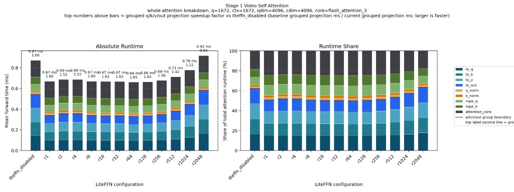
Results
Average Runtime
| Group | Transformer Mean (s) | Min (s) | Max (s) | Std (s) | Transformer % Faster | Decode Mean (s) | Save (s) | E2E Total (s) | E2E % Faster |
|---|---|---|---|---|---|---|---|---|---|
| baseline | 4.520 | 4.460 | 4.650 | 0.070 | 0.00% | 3.710 | 5.100 | 13.330 | 0.00% |
| litelinear | 3.500 | 3.490 | 3.520 | 0.010 | 22.57% | 3.710 | 5.100 | 12.310 | 7.65% |
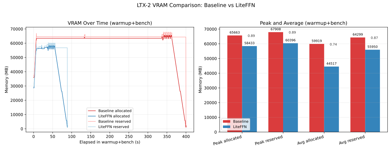
Allocated VRAM Reduction
| Configuration | Average | Peak | Peak Relative to Baseline |
|---|---|---|---|
| Original (FP16) | 59,919.00 MB | 65,663.00 MB | 100% |
| r=64 | 44,517.00 MB | 58,433.00 MB | 89.0% |
Video Samples (baseline vs LiteLinear r=32 / r=64 / r=512)
Click a thumbnail to play the video.
| Baseline | LiteLinear r=32 | LiteLinear r=64 | LiteLinear r=512 |
|---|---|---|---|
 |
 |
 |
 |
 |
 |
 |
 |
 |
 |
 |
 |
 |
 |
 |
 |
 |
 |
 |
 |
Quality Measurements
PSNR average over different seeds, per prompt (dB)[2] (Higher is better; 20 dB corresponds to a mean squared error of roughly 10−2):
| Prompt | baseline vs r=32 | baseline vs r=64 | baseline vs r=512 |
|---|---|---|---|
| a-dramatic-underwater-scene-featuring-a-person-s | 19.823 | 19.822 | 20.413 |
| a-man-in-a-sleek-modern-jetpack-flying-upwards-t | 20.872 | 21.517 | 21.163 |
| a-serene-view-of-the-banks-of-the-rhine-river-sh | 20.277 | 20.208 | 19.735 |
| a-single-water-droplet-falls-from-a-height-movin | 27.827 | 27.375 | 30.680 |
| two-anthropomorphic-cats-boxing-in-a-well-lit-ar | 18.646 | 20.924 | 21.188 |
Prompt PSNR Summary
| Prompt | Total seeds | PSNR > 20 dB | PSNR > 17 dB |
|---|---|---|---|
| a-dramatic-underwater-scene-featuring-a-person-s | 30 | 10 | 30 |
| a-man-in-a-sleek-modern-jetpack-flying-upwards-t | 30 | 30 | 30 |
| a-serene-view-of-the-banks-of-the-rhine-river-sh | 30 | 20 | 30 |
| a-single-water-droplet-falls-from-a-height-movin | 30 | 30 | 30 |
| two-anthropomorphic-cats-boxing-in-a-well-lit-ar | 30 | 20 | 30 |
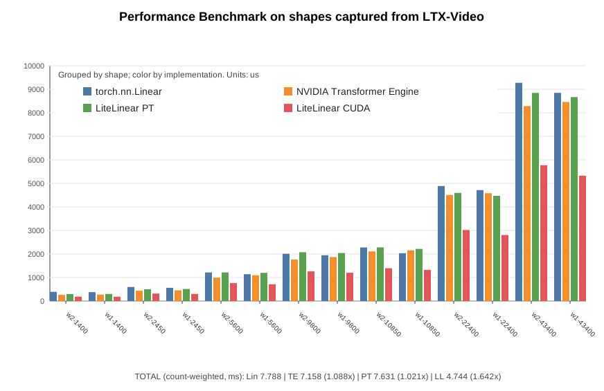
Performance of Synthetic Benchmark on Shapes Captured from LTX-Video
Multiplier columns are speedup ratios vs baseline linear (>1 faster, <1 slower).
Units:
- per-shape rows:
us TOTALrow:ms
Column glossary:
Cfg: FFN projection shape (w1= up-proj,w2= down-proj).M: flattened activation rows for that GEMM shape.Count: number of calls for that shape in the captured workload.Lin: baselinenn.Linearlatency.TE: Transformer Engine linear latency.PT: LiteLinear PyTorch path latency.CUDA: LiteLinear CUDA path latency.TE_x/PT_x/CUDA_x: speedup multiplier vs baseline linear (>1is faster,<1is slower).TOTAL: count-weighted aggregate across listed shapes.
| Cfg | M | Count | Lin | TE | PT | CUDA | TE_x | PT_x | CUDA_x |
|---|---|---|---|---|---|---|---|---|---|
| w2 | 1400 | 336 | 392 | 260 | 298 | 186 | 1.508x | 1.315x | 2.108x |
| w1 | 1400 | 336 | 378 | 273 | 301 | 182 | 1.385x | 1.256x | 2.077x |
| w2 | 2450 | 336 | 597 | 437 | 501 | 317 | 1.366x | 1.192x | 1.883x |
| w1 | 2450 | 336 | 562 | 455 | 511 | 302 | 1.235x | 1.100x | 1.861x |
| w2 | 5600 | 480 | 1213 | 994 | 1215 | 762 | 1.220x | 0.998x | 1.592x |
| w1 | 5600 | 480 | 1141 | 1097 | 1198 | 712 | 1.040x | 0.952x | 1.603x |
| w2 | 9800 | 144 | 2008 | 1763 | 2074 | 1261 | 1.139x | 0.968x | 1.592x |
| w1 | 9800 | 144 | 1946 | 1868 | 2042 | 1202 | 1.042x | 0.953x | 1.619x |
| w2 | 10850 | 336 | 2277 | 2110 | 2281 | 1395 | 1.079x | 0.998x | 1.632x |
| w1 | 10850 | 336 | 2035 | 2156 | 2215 | 1324 | 0.944x | 0.919x | 1.537x |
| w2 | 22400 | 144 | 4889 | 4506 | 4596 | 3018 | 1.085x | 1.064x | 1.620x |
| w1 | 22400 | 144 | 4714 | 4581 | 4471 | 2805 | 1.029x | 1.054x | 1.681x |
| w2 | 43400 | 144 | 9275 | 8285 | 8845 | 5772 | 1.119x | 1.049x | 1.607x |
| w1 | 43400 | 144 | 8847 | 8460 | 8669 | 5328 | 1.046x | 1.021x | 1.660x |
| TOTAL | - | 3840 | 7788 | 7158 | 7631 | 4744 | 1.088x | 1.021x | 1.642x |
Summary: LiteLinear CUDA implementation is 1.675x faster than torch.nn.Linear baseline across various shapes, captured from real video generation in LTX-Video. While the Linear implementation from Nvidia’s Transformer Engine is only 1.105x times faster.
Generalizing to Any DiT
The LTX-2 results are a proof of concept. The same technique applies to any Diffusion Transformer, because LiteLinear works at the nn.Linear level and requires no knowledge of the surrounding architecture. Candidates include:
- Other video DiTs, Wan2.1, CogVideoX, HunyuanVideo, Open-Sora, and others
- Image DiTs, Flux, SD3, PixArt
- World models and VLMs, any model with large feed-forward stacks
Beyond FFN: Attention Projections
LiteLinear targets not just FFN layers but also the Q, K, V, and O projection matrices inside attention. In LTX-2 (and most DiTs), these are Linear(dim, dim) layers, smaller than FFN projections but numerous. Compressing them adds incremental savings and, combined with FFN compression, can push total transformer runtime reduction above 30% on compatible hardware.
Attention projections are somewhat more sensitive to approximation error than FFN layers (since they participate directly in the softmax computation), so LiteLinear uses a more conservative default rank for them and allows independent rank control per layer type.
AMD GPU Support
LiteLinear supports AMD GPUs through ROCm, making it accessible to teams that operate AMD Instinct infrastructure (MI250, MI300, MI300X).
The core algorithm is calibration, SVD decomposition, and weight quantization. It is hardware-agnostic. The low-rank linear forward pass uses standard PyTorch operations that run on any backend. The FP8 remainder path uses ROCm's native FP8 tensor core support available on MI300-series hardware.
Version 0.3.0 stores remainders in AMD's native e4m3fnuz FP8 format. NVIDIA uses e4m3fn, so checkpoints are platform-specific: convert on the target GPU stack, or pass --fp8-dtype explicitly when cross-building. ROCm 6.3+ (rocm63 build flavor) is supported for 0.3.0; ROCm 7.2.0 and above remains the recommended stack.
AMD Acceleration Results
Synthetic Benchmark Results:
Cfg      M  Count |    Lin   ROCM |  ROCM_x
---------------------------------------------
w2     1400    336 |     312     265 |   1.177x
w1     1400    336 |     325     291 |   1.117x
w2     2450    336 |     536     411 |   1.304x
w1     2450    336 |     545     435 |   1.253x
w2     5600    480 |    1183     865 |   1.367x
w1     5600    480 |    1221     877 |   1.392x
w2     9800    144 |    2080    1507 |   1.380x
w1     9800    144 |    2052    1499 |   1.369x
w2    10850    336 |    2478    1626 |   1.523x
w1    10850    336 |    2345    1648 |   1.423x
w2    22400    144 |    4958    3374 |   1.469x
w1    22400    144 |    4976    3391 |   1.468x
w2    43400    144 |    9034    6547 |   1.380x
w1    43400    144 |    9655    6548 |   1.474x
---------------------------------------------
TOTAL        3840 |    8068    5700 |   1.415x
Result for LTX1 on 1280x720, 81 frames:
- 29% faster for FFN
- 6% faster E2E
Developer Guide
Version 0.3.0 separates offline conversion from runtime inference. Convert once with the lite-linear CLI, then load the resulting checkpoint into a model built with LiteLinear layers.
Installation
Pick a pre-built wheel from install/ that matches your Python version and GPU stack:
# 1) Clone the repository
git clone https://github.com/moonmath-ai/LiteLinear.git
cd LiteLinear

# 2) Install from a prebuilt wheel in install/ (pick Python + GPU flavor)
# NVIDIA (CUDA 12.8), Python 3.12, for example
pip install install/lite_linear-0.3.0+cu128-cp312-cp312-linux_x86_64.whl
Runtime dependencies (torch, safetensors) must be installed separately. The package is imported as lite_linear, and the lite-linear CLI is bundled in the wheel.
Quickstart: Convert Once, Load at Runtime
Step 1 — convert offline. The converter produces a distinct checkpoint artifact and never modifies the dense input file.
# Inspect layer keys and shapes
lite-linear inspect ltx-2.3-22b-dev.safetensors

# Decompose selected FFN layers (LTX-2 video + audio branches)
lite-linear convert ltx-2.3-22b-dev.safetensors \
    -o ltx-2.3-22b-dev-litelinear-r64.safetensors \
    --regex 'transformer_blocks\..*(audio_)?ff\.' \
    --rank 64
Each matched <prefix>.weight is replaced by four factor keys: <prefix>.A, <prefix>.B, <prefix>.Q_fp8, and <prefix>.Q_scale_inv.
Step 2 — wire LiteLinear in model source and load.
import torch
from safetensors.torch import load_file
from lite_linear import LiteLinear

# Replace target nn.Linear instances at construction time.
self.proj = LiteLinear(inner_dim, out_dim, bias=True, rank=64)

model = build_transformer_with_litelinear(...).cuda()
model.load_state_dict(
    load_file("ltx-2.3-22b-dev-litelinear-r64.safetensors"),
    strict=True,
)
model.eval()

x = torch.randn(1, seq_len, inner_dim, device="cuda", dtype=torch.bfloat16)
y = model(x)
Point your host pipeline at the converted file through the same checkpoint path, environment variable, or config entry you already use for model weights.
LTX-2 Two-Stage Distilled LoRA
When a distilled LoRA is applied at inference time, fuse it into the dense weights before decomposition so the low-rank factors represent the effective FFN weights:
lite-linear convert ltx-2.3-22b-dev.safetensors \
    --regex 'transformer_blocks\..*(audio_)?ff\.' \
    --lora ltx-2.3-22b-distilled-lora.safetensors \
    --lora-strength 0.8 \
    -o ltx-2.3-22b-dev-distilled-lora0.8-litelinear.safetensors
The converter applies W + strength * lora_B @ lora_A on matched layers, then decomposes the fused weight. Non-FFN layers can still receive runtime LoRA deltas from the dense checkpoint.
Autotune Cache (Cold-Start)
Kernel heuristic selection is cached separately from converted checkpoints. The default cache is ~/.cache/lite-linear/autotune_v13.cache on CUDA or ~/.cache/lite-linear/autotune_rocm_<arch>.cache on ROCm. Override with LITELINEAR_AUTOTUNE_CACHE_FILE=/path/to/cache.
Targeting Custom Layer Types
Use lite-linear inspect to discover module prefixes, then --regex or --manifest to select them. In model source, replace the corresponding nn.Linear with LiteLinear(..., rank=<same as convert>). For third-party hierarchies you cannot edit directly, walk named_modules() and match both nn.Linear and LiteLinear.
Removed in 0.3.0: model.eval() decomposition, LiteLinear.replace_activation_proj_, apply_lowrank_factors_to_transformer, load_lowrank_factors, and iter_ltx_ffn_linears. See MIGRATION.md if upgrading from earlier releases.
Rank Selection Guidelines
| Use case | Recommended rank |
|---|---|
| Maximum speed, modest quality | 32 |
| Balanced speed + quality | 64 |
| Near-lossless compression | 256, 512 |
| Per-layer adaptive | --manifest TOML with per-prefix ranks |
Hardware Requirements
| Platform | FP8 format | FP4 |
|---|---|---|
| NVIDIA H100 (Hopper) | e4m3fn | Planned (multiply-free) |
| NVIDIA B100/B200 (Blackwell) | e4m3fn | Yes (native) |
| AMD MI300X (ROCm) | e4m3fnuz | Planned |
Credit and Acknowledgments
LiteLinear builds on SVDQuant. Their work introduced the theoretical combination of low-rank decomposition with quantized remainders and calibration-aware effective weights. Our contribution is in taking those ideas to production: efficient CUDA/ROCm kernels, a scalable calibration pipeline, FP8 support, and generalization across layer types and model architectures.
We also thank:
- The Lightricks team for open-sourcing LTX-2
- The Flash Attention authors for pioneering efficient attention, which makes the remaining linear bottlenecks all the more important to address
References
- LiteLinear repository: https://github.com/moonmath-ai/LiteLinear
- SVDQuant Paper: https://arxiv.org/abs/2411.05007
- LTX-2: https://huggingface.co/Lightricks/LTX-2
- LTX docs: https://docs.ltx.video/welcome
Appendix: Mathematical Background
Singular Value Decomposition
SVD factorizes any matrix M into:
M = U @ S @ V^TU: orthogonal, columns are left singular vectorsS: diagonal, singular values sorted descendingV: orthogonal, columns are right singular vectors
Rapid decay of singular values means the matrix has low effective rank and can be well approximated with a small r.
Why Calibration-Aware Decomposition?
A naive SVD of W treats all input dimensions equally. But in practice, some dimensions are rarely activated. The autocorrelation matrix R = E[x x^T] captures which directions are important. Transforming W → W @ R^(1/2) down-weights unimportant directions before SVD, making the rank-r truncation much more accurate under real input distributions.
The square root is used because it "whitens" the input: transforming x → R^(-1/2) x gives identity covariance, so SVD operates in a normalized space where each component captures an equal share of variance.
Talk to us: research@moonmath.ai