

A Fast Attention Kernel for MI300X, Written in HIP, Not Assembly
A deep dive into building a bf16 forward attention kernel for AMD MI300X in HIP, using instruction level control without dropping into a full assembly codebase.
TL;DR
- A bf16 forward attention kernel for AMD MI300X, written in HIP rather than full hand assembly.
- The core technique is one-instruction asm wrappers: choose exact opcodes while leaving register allocation to the compiler.
- The design plans the CDNA3 pipeline directly: eight waves, two groups, and two carefully placed barriers.
- Most of the speedup comes from memory placement:
KinLDS,Vkept hot inL1,Qand accumulators in registers. - 3Q tiling and the tail KV split turn a near tie into wins across the reported sweep.
- Code is open-source under MIT and can be found here.
- We would like to thank HotAisle, our AMD cloud, for bare metal access and general support.
A bf16 forward attention kernel for AMD MI300X (gfx942), written in HIP rather than assembly, that beats AITER v3 on every shape and every rounding mode. Geomean 1.18×, 1.15×, 1.08× (RTNE, RTNA, RTZ), up to 1.26×, across an 8K to 128K sweep, and 1.37× to 1.59× versus Modular MAX.
1. What we built, and the idea behind it
Attention is the fused softmax(QKᵀ/√d)·V operation at the core of every transformer. As part of our kernel engineering work, we built a full BF16 forward-attention kernel for AMD MI300X (CDNA3, gfx942). In our benchmarks, it outperformed the best existing AMD implementation on MI300X. This write-up provides the technical details, lessons, and some techniques we found useful and can be reused.
AITER is AMD's own optimized kernel library, and its v3 forward attention is written by hand in GCN assembly. Against it, our kernel wins on every shape and every rounding mode across an 8K to 128K token sweep. The geomean is 1.18×, 1.15×, 1.08× for RTNE, RTNA, and RTZ rounding, and 1.37× to 1.59× against Modular MAX. RTNE and RTNA lead by 1.11× to 1.26×. RTZ is AITER's own fastest mode, the tightest race, and there we win by a slimmer 1.03× to 1.11×.
For a rigidly structured computation like attention, the way to win is to make the scheduling decisions yourself instead of leaving them to the compiler. The compiler's job is to be a good generalist, and a fused attention kernel is not a general program. It is a pipeline whose exact shape we already know, down to which instruction should issue when, what should be in flight, and where each barrier goes. Almost every section here takes one of those decisions in hand. There is one honest exception, in §3.1, where the smarter move is the opposite: hand the compiler an easier problem and let it do the overlap itself. We flag it when we get there.
This blog post is structured as follows: the toolkit (§2) is the handful of barely documented techniques that make instruction level control possible from HIP at all. The architecture (§3) covers why eight waves, how the two halves overlap, and which matrix core instruction we use and why. The memory hierarchy (§4) is what lives in registers, LDS, and L1, and the lengths we go to to keep it there. The two advanced wins (§5) turn a near tie into a clean sweep. The full results are in §6.
2. The toolkit
2.1 Templated asm functions
Everything that follows rests on one technique, and it is the one we found least documented anywhere, so we start here.
Every HIP kernel author hits the same dilemma when they want a specific machine instruction. Compiler intrinsics (__builtin_amdgcn_*) keep you in tidy C++, but the compiler then feels free to help in ways you did not ask for. It may rename your accumulator into a fresh register and add a v_mov to copy it back, re-zero an operand you know is already zero, or reorder the instruction against its neighbours. Drop to raw inline assembly and you get exactly the instruction you asked for, but AMD's own guidance is blunt about the price: inline asm is "not recommended, since the compiler does not look at the semantics of the inlined instructions, and may not take care of data hazards" (AMD matrix cores lab note). And now you are managing registers and addresses by hand too.
The way through is a small pattern. Wrap exactly one instruction in a __device__ __forceinline__ function and describe its operands with GCC or Clang extended asm constraints. You dictate the opcode, and the compiler still allocates the registers and tracks the data flow.[1] Here is the MFMA we issue hundreds of thousands of times:
// in/out tied to the SAME VGPR → no accumulator rename, no v_mov copy.
__device__ __forceinline__ void asm_mfma(bf16x4_t a, bf16x4_t b, fp32x4_t& c) {
    asm volatile("v_mfma_f32_16x16x16_bf16 %0, %1, %2, %0"
                 : "+v"(c) : "v"(a), "v"(b));
}
The whole trick is in the constraint string. "+v"(c) says that c is a read-write VGPR operand, so the accumulator's input and output land in the same register and the compiler emits no copy. "v"(a) and "v"(b) are VGPR inputs it places wherever it likes. A sibling, asm_mfma_zero, feeds a literal 0 as the C operand and declares its result "=&v", write only and early clobber, to start a fresh accumulator chain without even the zeroing v_mov.
The same pattern folds compile time constants into the instruction. Our paired LDS read takes its two offsets as template parameters and emits them as literals:
template <int kOffset0, int kOffset1>
__device__ __forceinline__ u32x4_t ds_read2_b64_imm(uint32_t lds_base) {
    u32x4_t result;
    asm volatile("ds_read2_b64 %0, %1 offset0:%c2 offset1:%c3"
                 : "=&v"(result) : "v"(lds_base), "i"(kOffset0), "i"(kOffset1));
    return result;
}
"i" marks an immediate and %c emits the bare number, so the offsets become part of the opcode. A single compiler allocated base register (lds_base) serves every read, and the per read offset costs zero registers and zero address math. The & in "=&v" (early clobber) tells LLVM not to reuse the result's register for any input, the exact guarantee that keeps the load from stomping its own address. (Full constraint vocabulary is in the LLVM Language Reference.)
That is the keystone. One instruction per wrapper keeps AMD's hazard warning contained, the constraints hand register allocation back to the compiler, and we still choose every opcode that matters.
The net effect is the one we kept coming back to. You write HIP, ordinary functions, variables, and templates, with zero register or address bookkeeping, and yet you steer the machine one instruction at a time. You get to have the cake and keep it whole. It is striking how much of the field skips this middle path. AITER's v3 forward attention, our strongest baseline, is written by hand in GCN assembly, as are plenty of other heavily tuned kernels, all paying the full price of authoring and maintaining raw asm. We beat them (§6) from code that stays much closer to ordinary HIP, not by working harder at the assembly but by largely not having to.
Sometimes the payoff is even correctness rather than speed. We will hit a case in §2.2 where the intrinsic form silently drops writes. The rest of the kernel is written in this vocabulary.
2.2 Asynchronous memory and synchronization
§2.1 picks the instructions. This section is about what goes between them. The speed comes from keeping several memory pipes busy at once, K streaming from HBM into LDS, LDS reads feeding the QK matmul, and V loads from L1, so one wave group's matrix core work hides the other's memory latency. On CDNA3 those loads are asynchronous. A load issues and returns right away, and the hardware tracks completion in two counters, vmcnt for vector memory such as global and buffer loads, and lgkmcnt for LDS. Nothing stalls until you wait on a counter.
So the whole game is to arrange never to actually wait. We keep enough loads in flight that by the time the matrix core needs a value it has already arrived. The LDS reads feeding each matmul are issued well ahead and kept outstanding, double buffered and never drained to zero, so a matmul consumes data that landed cycles ago instead of stalling on a fresh read. The matrix core never waits on LDS.
And it is not one pipe but several, all in flight at once. While the matrix core is consuming this iteration's tiles, reading K from LDS and V from L1 into registers, the kernel is already fetching the next iteration's data: the next K block streaming from HBM into LDS, and the next V tile prefetched into L1, both asynchronous and both overlapped with the current compute. By the time one iteration ends, the next one's data is already on chip, so the matrix core runs straight from one iteration into the next, never loading on demand.
This is exactly why the obvious HIP tool is the wrong one. __syncthreads() drains all outstanding LDS traffic and raises a workgroup barrier in a single stroke, emptying the very pipes we work to keep full. And the GFX942 memory model says a full LDS drain is only needed to synchronize LDS against vector memory between wavefronts, "not between operations performed by the same wavefront" (LLVM Memory Model GFX942). So in place of one heavy barrier we order the memory with lightweight counter waits, each leaving the right number of loads in flight, and use a real s_barrier only at the two points each iteration must synchronize, the phase handoff in the middle and the iteration boundary (§3.2).
That is the discipline. §2.1 chooses each instruction, and §2.2 keeps every pipe full and waits only where the data is genuinely needed. Neither is something the compiler will do for a schedule we built ourselves, which is why the next thing we needed was a way to see the schedule it actually produced.
2.3 The profiler feedback loop
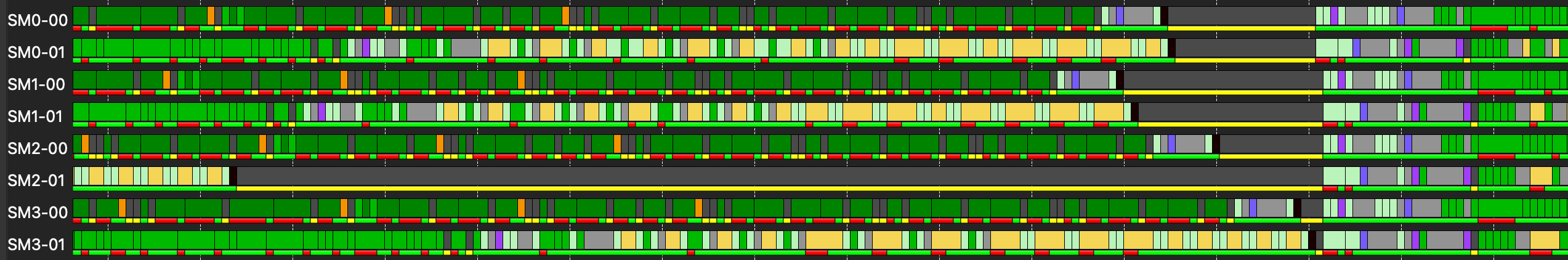
Placing waits and barriers by hand is guesswork unless you can see what the hardware actually did with them. Our feedback loop was the ROCprof Compute Viewer. You capture a thread trace (ATT) with rocprofv3, and the viewer renders it as a per SIMD timeline. For every SIMD it shows which pipe, matrix core, VALU, LDS, or vector memory, is busy in each window, with every instruction mapped back to the compiled ISA and annotated with a hitcount and latency.
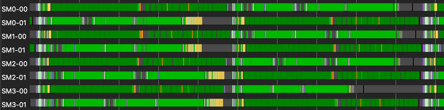
That view settles the questions §2.1 and §2.2 raise but cannot answer on their own. Is Group A's MFMA actually overlapping Group B's K load, or are they accidentally serialized? Did a wait drain a pipe a few cycles too early and leave the matrix core idle? Did the compiler sink a prefetch past a sched_fence? Each shows up as a gap in the timeline. You trace the gap to the instruction and know exactly which wait, barrier, or priority hint to move.
So the real workflow was never write then hope. It was a loop.[2] Most of the kernel's structure, the Group A and Group B phase split, the prefetch ring depths, and where the two per iteration barriers sit, was found by staring at the timeline until the gaps closed.
3. The architecture
The kernel is built around one move: keep the matrix core busy while the memory work happens in its shadow. Everything that follows serves that, beginning with a choice that sounds mundane but decides the rest, how many waves go in a block.
3.1 Why 8 waves per block
A CDNA3 compute unit has four SIMD units, so the textbook block is four waves, one per SIMD, and you lean on the compiler to keep the hardware busy by running several such blocks per CU at once and interleaving their memory and compute (MI300 workload optimization). It works, but it hands the scheduling decisions that matter most to occupancy heuristics. For attention, a rigidly structured dataflow, we wanted those decisions ourselves, so we run eight waves per block, two groups of four, one wave per SIMD per group.
Three reasons.
Overlap, the easy way. More resident waves give the compiler more independent instruction streams to interleave, so it keeps the matrix core fed and hides the individual instruction latencies on its own, without us scheduling each instruction by hand. That the compiler needs the help is visible all through the kernel, in the scheduling workarounds of §2.1 and §2.2: source order MFMA issue, pinned waits, and sched_fence. Wave count is the one lever that helps the compiler here without dropping to assembly, the single place in this whole story where we make its job easier instead of overriding it.
One copy of K in LDS, V in L1. Every wave's QK matmul reads the same K tile from LDS, and every PV reads the same V_t tile, kept resident in L1 (§4.3). Eight waves in one block share that single K allocation. Two independent four wave blocks would each stage their own copy of the same K tile. Moving V off LDS entirely freed even more room, exactly what we later spent on the 3Q trick (§5.1).
A pipeline we plan, not one we hope for. Owning all eight waves in one block lets us assign fixed roles, one group of four on the matrix core, the other on memory and softmax, and switch them in lockstep. With the compiler scheduling separate blocks on its own there is no stable structure to plan against. With one block we own, there is. That schedule is the next section.
3.2 Overlapping compute and memory
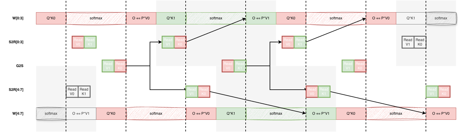
The two groups of §3.1 are symmetric. Both run the full Q*K, softmax, O += P*V sequence on their own q tiles. We simply offset them by a phase, so that while one group is on the matrix core the other is in softmax and issuing the next loads, then the reverse. Each K block iteration has two phases, and the groups trade which job they hold between them:
                 Group A                       Group B
  Phase 1   pv[N-1] + qk[N]            K[N+1] HBM→LDS  +  softmax[N-1]
  Phase 2   softmax[N] + V_t prefetch  pv[N-1] + qk[N]
At every moment one group is saturating the matrix core, the pv and qk MFMAs, while the other does the work that is not matrix core work. Then they swap, so the matrix core never idles waiting on memory. K lives in a double buffered LDS allocation, two halves, so the block being consumed in QK and the block being loaded for the next iteration never collide.
It is worth contrasting this with FlashAttention-3 on Hopper, because the resemblance is shallower than it looks. FA3 leans on warp specialization. A separate producer warp group does nothing but issue asynchronous copies while other warp groups run the matmuls (FlashAttention-3). That division of labour pays off on NVIDIA, but on CDNA3 we found it usually does not. Every memory move here is already asynchronous (§2.2), so you issue a load, it travels on its own, and a counter tells you when it landed. There is no reason to sacrifice a whole wave to moving data. Both of our groups issue their own loads and keep computing softmax right through. The one part of FA3 we really echo is the alternation of matmul and softmax across groups, not the producer and consumer split.
The hard part is the synchronization, and it really is an art. There are two s_barriers per iteration, one in the middle at the phase 1 to phase 2 handoff, and one at the iteration boundary, the latter an lds_barrier that drains the LDS side with lgkmcnt(0), alongside the targeted vmcnt(0) wait from §2.2 that lands the K writes. One barrier too many and the groups stop overlapping. One too few, or in the wrong place, and a group reads a tile the other has not finished writing. Placing both barriers correctly, and trusting the per counter waits to do the rest, is most of what made the pipeline fast, and it is exactly what the §2.3 timeline let us tune.
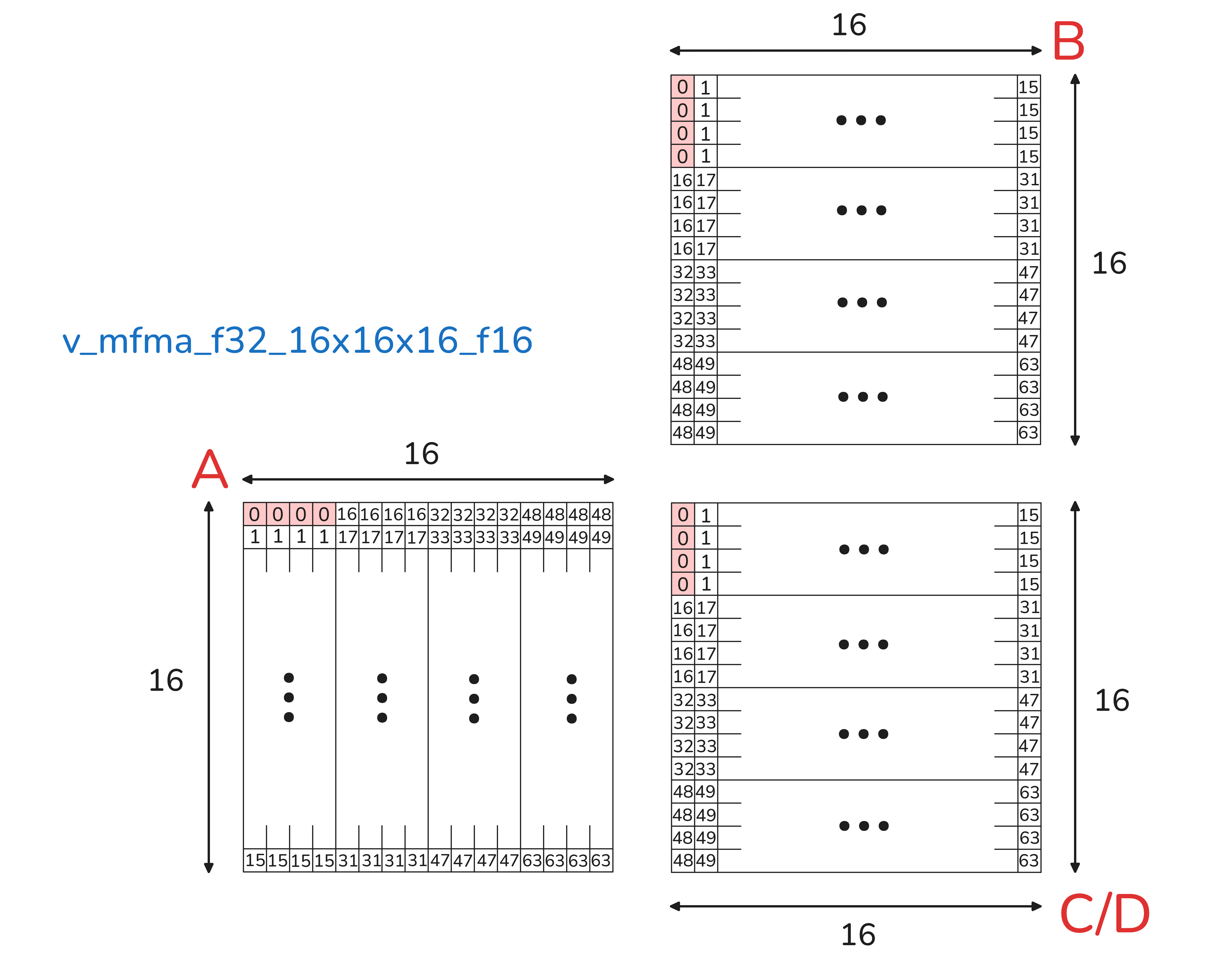
3.3 Why 16×16×16, not 32×32×8
CDNA3's matrix cores offer several bf16 MFMA shapes, and the natural candidates for attention are 32×32×8 and 16×16×16. They have identical matmul throughput, both 512 flops per cycle per CU,[3] so the choice is not about raw speed. It is about everything around the instruction.
The deciding factor is register footprint. A 16×16×16 accumulates into just 4 fp32 elements per lane, since our scores and o_acc fragments are fp32x4, while 32×32×8 holds 16 per lane.[4] Four wide fragments mean far less accumulator VGPR pressure, leaving registers for deeper prefetch rings and persistent Q, and fewer accumulator register file writes per instruction, which is where the lower energy comes from. AMD's own MI300X tuning guide makes the same call, noting that "MI16x16 outperforms MI32x32 due to its superior power efficiency" (MI300X workload tuning guide). The K and V operands are smaller per instruction too, so we stream them from LDS in tight, frequent reads instead of holding large fragments.
There is a structural payoff as well. A 16 row tile (M = 16) means Q composes in 16 row units, and that granularity is precisely what lets us run three 16 row Q tiles per wave, 48 rows, in §5.1. A 32 row tile cannot take that step.
The cost is bookkeeping. Smaller tiles mean more of them, and the lane to fragment index math gets fiddly fast. We keep it tractable two ways. First, compile time layout maps, where an index is Σ coordᵢ·strideᵢ that the compiler folds to shifts rather than arithmetic we write by hand. Second, AMD's Matrix Instruction Calculator, which prints the exact element, register, and lane mapping we validate every fragment layout against. That is how you address the matrix core at this granularity without drowning in indexing.
4. The memory hierarchy
4.1 What lives where
MI300X gives each compute unit a 512 KiB vector register file, 64 KiB of LDS, and a 32 KiB L1 vector cache, over a 32 MiB shared L2 and 256 MiB Infinity Cache.[5] The whole kernel is, in a sense, one long argument about which of those holds what. Our answer:
| Data | Lives in | Why |
|---|---|---|
Q tile |
VGPRs, persistent, LDS partially |
Read every iteration, never reloaded. |
| Output and scores | VGPRs, fp32 accumulators | Matrix core outputs never leave registers until the final store. |
K tile |
LDS, double buffered, 32 KiB |
Shared by all 8 waves, one copy, swapped per iteration. |
V tile, V_t |
L1, resident |
Shared and reread across the PV matmul, kept hot deliberately. |
Two consequences set up the rest of this section. K and V take different paths into the CU, K streamed into LDS and V pulled from L1, and keeping them apart is what stops one from evicting the other (§4.2, §4.3). And K's double buffer is exactly 32 KiB, half the CU's 64 KiB, with the other half spent on a third Q tile (§5.1). One grid level decision rounds it out. A head first chiplet swizzle maps all of a (batch, head)'s q blocks onto a single XCD, so its K and V stay resident in that XCD's slice of L2 instead of thrashing across all eight.
4.2 Swizzling K into LDS
K reaches the matrix core by the most direct route the hardware allows. An async buffer_load_dword … lds, the load we wrote by hand in §2.2, streams it from HBM straight into LDS, with no value ever passing through a VGPR. That keeps K out of the vector registers we need for Q and the accumulators, and off L1, so it cannot evict the V tile we keep hot there (§4.3).
Once in LDS, K has a bank conflict problem. A K row is 64 dwords, and LDS has 32 banks of 4 bytes, so a 64 dword stride is 0 mod 32. Every row starts in the same bank, and the column reads the QK matmul issues all collide. The textbook fix is to pad each row to 66 dwords so successive rows step across banks, and an earlier version of the kernel did exactly that. But padding costs the very LDS we cannot spare. With the third Q tile (§5.1) the budget is exactly 32 KiB of K plus 32 KiB of Q, which fills the 64 KiB, with no slack for a 3% pad, and padding measured slower besides.
So the K row stays a dense 64 dwords and we break the conflict with an XOR swizzle, a zero storage permutation of where each dword lands. The key is to apply the same swizzle twice so it cancels, once on the write from HBM into LDS, so each lane deposits its dword at a swizzled slot, and again folded into the QK read address:
// QK read base. Fields are bit disjoint, so the OR is just an add. (quad ^ col_lo) swizzles.
const uint32_t qk_swz_base = (col << 8) | ((quad ^ col_lo) << 3);
Because the fields are bit disjoint the OR is a free add, with no extra instruction and no extra register. And the swizzle is designed to leave the §2.1 immediate offset read intact. The constant d tile pair offset still rides the ds_read2 … offset1:16 immediate, so one op fetches both d tiles, and only the variable d tile index moves into the swizzled base. We get conflict free LDS, zero padding, and still pay nothing per read.[6] (AMD documents both padding and XOR swizzle for this.)
4.3 Keeping V in L1
V takes the opposite path. Rather than staging it through LDS like K, we keep the pre transposed V tile resident in L1 and read it from there on every PV matmul. The catch is that unlike LDS, L1 is not a memory you can address. You cannot put something in L1, you can only load through it and hope it stays. So keeping V in L1 has to be engineered indirectly.
We do it by prefetching. In the phase where one wave group is busy with softmax and nothing else (§3.2), the other group fires a wave of loads for the next iteration's V tile, split so its four waves request sixteen distinct cache lines at once and hit all of L1's sets in parallel, into a throwaway register the next instruction overwrites. The data is never used. The point is the side effect. The lines land in L1, so when the PV matmul reads them an iteration later they are already hot.
This is the part of the design that leans hardest on understanding the hardware rather than the manual, the same empirical tradition of microbenchmarking the cache that earlier work applied to NVIDIA GPUs (Jia et al.) and to AMD's consumer parts. There is no API that says to pin this in L1. There is a load pattern that, once you know how the cache behaves, reliably leaves it there.
4.4 Why V gets its own kernel
There is a detail hiding in §4.3. We keep V_t in L1, that is V already transposed and repacked, not raw V. The reason is the score matrix. One matmul writes it, softmax reduces it, the next matmul reads it, and its orientation is a single choice all three have to share. We make that choice for the softmax: computing the scores as K·Qᵀ rather than the textbook Q·Kᵀ lines the keys up along each lane's own registers, so the per query max and sum reduce locally instead of sweeping the whole tile. The price falls on the second matmul: to multiply against scores laid out that way, it needs V transposed to match. And since V is a fixed input we reread every iteration, we pay that transpose once, in a separate kernel that runs before attention and earns its place two ways.
The first is layout. The matrix core wants each lane's MFMA input as a specific, scattered selection of V's elements. Load raw V and every lane has to gather and permute its fragment after the load, on the critical path, every iteration. Instead the transpose kernel writes V in exactly the order the PV matmul consumes, so each lane issues a single contiguous 16 byte load, two MFMA operands, with no shuffle, broadcast, or permute afterward. We cross check that order against AMD's Matrix Instruction Calculator, which spells out the exact element, lane, and register mapping the instruction expects.
The second is L1. Doing the repack inline would mean pulling V through the vector registers to reorder it, the very VGPR pressure and L1 traffic that §4.2 and §4.3 work to avoid. As a standalone pass it lands V_t in memory once, laid out so the attention kernel only ever reads it, straight from L1.
We do not force the cost on callers. It is a separate launch today, for a drop in API. But it could be folded into the contract, requiring pre transposed V, and the runtime transpose would vanish entirely. The repack also zero pads V_t to a 64 row boundary, so a partial last block contributes a clean 0 rather than garbage, a small correctness nicety that falls out of owning the layout.
5. The advanced wins
5.1 The 3Q tile increase
Recall the LDS budget from §4.1. K's double buffer is 32 KiB, and moving V to L1 (§4.3) left the other 32 KiB of the CU's 64 KiB free. The 3Q increase spends it.
A wave processes Q in 16 row tiles. The earlier design carried two tiles per wave, 32 rows, entirely in registers. We add a third, QTilesPerWave = 3, 48 rows per wave and 384 per workgroup, but the third tile cannot go in registers, since the VGPR file is already full of accumulators and K and V fragments. So it lives in the freed 32 KiB of LDS instead:
constexpr int QTilesPerWave = 3;            // → 48 q-rows / wave
__shared__ uint32_t lds_q2[Q2LdsDwords];    // 32 KB: the whole third Q tile
The first two tiles stay VGPR resident and hot. The third is parked in LDS up front and streamed through a small ping pong buffer during the QK matmul. Crucially, its LDS reads, tracked by lgkmcnt, overlap the V loads from L1, tracked by vmcnt, so the extra traffic hides behind work already in flight instead of adding latency. The two halves of LDS now add up exactly, 32 KiB of double buffered K plus 32 KiB of third Q tile, the full 64 KiB.
Why bother? More Q rows resident per workgroup means each K and V tile we load is reused across 50% more queries before eviction, the same data reuse lever FlashAttention pulls with tiling (FlashAttention), pushed as far as the LDS allows. That extra reuse is most of the jump from the two tile kernel's roughly 1.04× over AITER to 3Q's geomean 1.14×, 1.10×, 1.02× (RTNE, RTNA, RTZ).
It does not quite win everywhere yet. Three RTZ shapes still trail AITER by about 5%. That is what the next section fixes.
5.2 The tail KV split
MI300X has 304 CUs, and 304 is an awkward number. Our workgroups run in rounds of 304, so when the grid does not divide evenly the last round is a fraction of a round. The CUs without a workgroup sit idle while the stragglers each still walk the entire K and V sequence. On a long context shape that stranded round can dominate the runtime.
The fix is borrowed straight from Flash-Decoding (Dao et al.). When there is a tail, split it. The CTAs in the stranded round each own one Q block, and we slice their K and V range into G parts and hand each to a different idle CU, so the whole machine attacks the tail at once instead of a handful of CUs grinding through it serially. Each part computes a partial output plus its softmax statistics, the running max m and denominator l, and a small merge_parts kernel recombines them with the standard online softmax rescale (weight = exp2(mₚ − max)), the exact log sum exp merge Flash-Decoding uses.
What is ours is the planning. A split only pays off sometimes, so a host side cost model picks G, or declines. It weighs the rounds saved against the merge overhead and bails when the grid already divides evenly, when the last round is at least 95% full, or when the sequence is too short for the merge to earn its keep.
const int tail = wgs % NumCUs;   // CTAs in the stranded final round (NumCUs = 304)
// pick G minimizing  ceil(tail·G / 304) rounds × ceil(nkb / G) blocks per part  + merge
The same arithmetic lives in tools/tail_speedup.py, so a shape's speedup is predictable before you run it. This split is what erases the last RTZ losses from §5.1. (4,16,16384) RTZ goes from 0.95× to 1.07×, taking the kernel to a win on every shape and every rounding mode, geomean 1.18×, 1.15×, 1.08× versus AITER (§6).
There is a sibling trick on the sparse and lite path, an LPT (longest processing time) reordering that runs the heaviest q blocks first, but that is a separate mechanism for a different kernel. Here we mean the dense split.
6. Results and takeaways
Measured on MI300X, bf16, with head dimension 128 throughout. Each row is one input shape (B, H, S, D), for batch, heads, sequence length, and head dimension, at one rounding mode. The rounding mode sets how the fp32 matmul accumulators are packed back to bf16: RTNE rounds to nearest even, RTNA rounds to nearest with ties away from zero, AITER's default, and RTZ truncates toward zero. We match AITER's rule in each mode. Speedup is other_ms / ours_ms, so a value above 1× means we are faster. Times are the median of 5 passes of 30 iterations on an idle GPU. Our kernel accepts inputs in either [B, S, H, D] (BSHD, the diffusion style layout) or [B, H, S, D] (BHSD), with no transpose either way. The baselines are AITER, specifically its v3 forward attention written in assembly, and Modular MAX. MAX has no rounding mode selector and rounds RTNE internally, so its column is identical across the three modes.
| Shape (B, H, S, D) | Round | Ours (ms) | AITER v3 (ms) | Speedup vs AITER | Modular MAX (ms) | Speedup vs MAX |
|---|---|---|---|---|---|---|
| (2, 24, 8192, 128) | RTNE | 3.083 | 3.792 | 1.23× | 4.237 | 1.37× |
| (2, 24, 8192, 128) | RTNA | 3.022 | 3.605 | 1.19× | 4.237 | 1.40× |
| (2, 24, 8192, 128) | RTZ | 2.983 | 3.303 | 1.11× | 4.237 | 1.42× |
| (2, 24, 16384, 128) | RTNE | 11.670 | 14.691 | 1.26× | 17.923 | 1.54× |
| (2, 24, 16384, 128) | RTNA | 11.479 | 13.801 | 1.20× | 17.923 | 1.56× |
| (2, 24, 16384, 128) | RTZ | 11.385 | 12.629 | 1.11× | 17.923 | 1.57× |
| (1, 32, 16384, 128) | RTNE | 8.013 | 9.031 | 1.13× | 11.030 | 1.38× |
| (1, 32, 16384, 128) | RTNA | 7.828 | 8.656 | 1.11× | 11.030 | 1.41× |
| (1, 32, 16384, 128) | RTZ | 7.731 | 7.989 | 1.03× | 11.030 | 1.43× |
| (4, 16, 16384, 128) | RTNE | 15.591 | 18.337 | 1.18× | 22.061 | 1.41× |
| (4, 16, 16384, 128) | RTNA | 15.331 | 17.567 | 1.15× | 22.061 | 1.44× |
| (4, 16, 16384, 128) | RTZ | 15.055 | 16.183 | 1.07× | 22.061 | 1.47× |
| (1, 64, 16384, 128) | RTNE | 15.528 | 18.333 | 1.18× | 22.763 | 1.47× |
| (1, 64, 16384, 128) | RTNA | 15.239 | 17.535 | 1.15× | 22.763 | 1.49× |
| (1, 64, 16384, 128) | RTZ | 15.040 | 16.161 | 1.07× | 22.763 | 1.51× |
| (2, 24, 32768, 128) | RTNE | 46.002 | 54.794 | 1.19× | 69.947 | 1.52× |
| (2, 24, 32768, 128) | RTNA | 44.440 | 52.363 | 1.18× | 69.947 | 1.57× |
| (2, 24, 32768, 128) | RTZ | 44.075 | 48.549 | 1.10× | 69.947 | 1.59× |
| (2, 16, 65536, 128) | RTNE | 117.612 | 136.301 | 1.16× | 171.273 | 1.46× |
| (2, 16, 65536, 128) | RTNA | 115.550 | 130.278 | 1.13× | 171.273 | 1.48× |
| (2, 16, 65536, 128) | RTZ | 114.665 | 121.668 | 1.06× | 171.273 | 1.49× |
| (2, 8, 86016, 128) | RTNE | 101.071 | 118.939 | 1.18× | 141.319 | 1.40× |
| (2, 8, 86016, 128) | RTNA | 100.165 | 114.515 | 1.14× | 141.319 | 1.41× |
| (2, 8, 86016, 128) | RTZ | 99.397 | 106.513 | 1.07× | 141.319 | 1.42× |
| (1, 16, 131072, 128) | RTNE | 232.517 | 269.278 | 1.16× | 339.322 | 1.46× |
| (1, 16, 131072, 128) | RTNA | 228.475 | 258.092 | 1.13× | 339.322 | 1.49× |
| (1, 16, 131072, 128) | RTZ | 226.152 | 239.587 | 1.06× | 339.322 | 1.50× |
Across all shapes the geomeans are:
| Rounding mode | Geomean vs AITER | Geomean vs MAX |
|---|---|---|
| RTNE | 1.18× | 1.44× |
| RTNA | 1.15× | 1.47× |
| RTZ | 1.08× | 1.49× |
The row we are proudest of is the narrowest. RTZ is AITER's own fastest variant, so beating it at all, let alone on every shape, was the hardest part of the claim, and for most of the project we did not. The 3Q kernel still lost three RTZ shapes by about 5% (§5.1). The tail split (§5.2) is what turned those last losses into wins. A clean sweep came down to the last few idle CUs.
What we would take away. Four things, and they are the same four sections:
- You can have instruction level control without writing the kernel in assembly. The whole thing is HIP. The leverage is a handful of one instruction asm wrappers (§2.1) that let the compiler keep doing register allocation while we pick the opcodes. AITER's v3 is assembly written by hand, far more code and far more to maintain, and we beat it from something much closer to ordinary HIP. That middle path is badly underused.
- Plan the pipeline, do not hope for it. For a computation whose shape you know exactly, attention being the canonical case, the compiler's general purpose scheduling is a worse bet than a layout you design yourself (§3): eight waves, two groups, two barriers.
- Optimization is mostly a memory placement argument. Where K, V, Q, and the accumulators live, and the lengths you go to keep them there (§4), decided more of the speedup than any single instruction did.
- Optimizations cascade. Moving V to L1 freed the LDS that paid for a third Q tile, which forced K's swizzle, which had to preserve an addressing trick from three sections earlier (§4.2, §5.1). The wins were never independent. Each reshaped the constraints for the next.
If the whole effort reduces to a single idea, it is this: we give the compiler a structured framework, built by hand, so that it can do what it does best, optimize locally within it.
SGLang integration
We added LiteAttention support to the attention kernel. We used this AMD kernel to optimize video diffusion models via a PR to SGLang diffusion: on Wan-AI/Wan2.1-T2V-1.3B-Diffusers, switching the transformer attention from AITER to liteattention_rocm improved end-to-end video generation time by 1.23× on MI300X (gfx942), with no visible quality regression.